
Over the last few weeks I have been reading What Every Programmer Should Know About Memory by Ulrich Drepper and the chapter on Optimizations from 100 Go Mistakes and How to Avoid Them, this is a summary of what I've learned from them. I would highly recommend you read the paper for yourself, it will help you understand the hardware better, in-turn helping you write better software.
First, a simple vizualiztion of what the CPU, Cache and Memory are linked together:
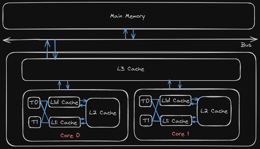
L1d Cache
As a programmer you will get the highest performance yield by focusing on the level 1 cache. That will be the focus of this short summary. I might write about improving the other levels in another article. Obviously, all the optimizations for the level 1 cache also affect the other caches.
The theme for all memory access is the same: improve locality (spatial and temporal) and align the code and data.
Spatial Locality
Also, known as locality in space.
The principle of spatial locality says that if a program accesses one memory address, there is a good chance that it will also access other nearby addresses.
Example: in an array, items are stored contiguously in memory
Temporal Locality
It is also known as locality in time.
The principle of temporal locality says that if a program accesses one memory address, there is a good chance that it will access the same address again.
In the code below, sum and i are repeatedly read from and written to. The function someFunc, could be located elsewhere in the address space but calls to the function are close in time with sum and i.
sum := 0
for i := 0; i < Max; i++ {
    sum += someFunc(i)
}
What about L1i?
There are a few reasons, why we are focusing on the L1d over L1i:
- The quantity of code which is executed depends on the size of the code that is needed. The size of the code in general depends on the complexity of the problem. The complexity of the problem is fixed.
- While the program’s data handling is designed by the programmer the program’s instructions are usually generated by a compiler.
- Program flow is much more predictable than data access patterns. Modern CPUs are very good at detecting patterns. This helps with prefetching.
- Code always has quite good spatial and temporal locality.
Although, I might write a seperate article on making the most of L1i.
Performance Comparison between various levels of cache
The closer the cache is to the CPU the smaller it is in size and access times are exponentially faster. Here are some rough comparison between various cache levels.
| Cache | Cycles | Size |
|---|---|---|
| Register | <1 | Between 64 Bits and 512 Bits |
| L1d | ~3 | Between 32 KB and 512 KB |
| L2 | ~14 | Between 128 KB and 24 MB |
| L3 | ~40 | Between 2 MB and 32 MB |
| Main Memory | ~100-300 | Between 1 GB and 128+ GB |
You can check the cache size on your machine by running:
lscpu | grep cache
Although, the cost of access is quite high, beyond the L1d, the CPU hides some of this cost by parallelly loading data when possible.
Cache Lines
Entries stored in cache are not single words (unit of data transferred between the CPU and the cache) but "lines" of several contiguous words. You can check your cache line size by running:
getconf LEVEL1_DCACHE_LINESIZE, on my machine it's 64 bytes long.
We cannot talk about cache lines and not mention associativity. There are three main types of associativity:
1. Fully Associative Cache
Cache is fully associative when each cache line can hold a copy of every memory location. To access an entry the processor would have to compare the tags of every cache line to find the requested address, which can become quite slow or expensive.
So they are only used in the Translation Lookaside Buffer(TLB) where those caches are really small with only a few dozen entries.
2. Direct-Mapped Cache
Here each tag maps to exactly one cache entry. This is fast and relatively easy to implement but has a major drawback. It only works well if the addresses used by the program is evenly distributed. Usually, this is not the case. So what ends up happening is either a frequently required resource is evicted from the cache repeatedly or cache entries are hardly used or remain empty.
3. Set-Associative Cache
This approach takes the best of both the approaches above. Set-Associativity greatly reduces the number of cache misses. Also, up to a certain number of sets, introducing associativity has the same effect as doubling cache size.
Example: For an 8MB cache going from direct to 2-way set associative cache saves almost 44% of the cache misses.
Computing Memory address for cache line
When the contents of memory are needed the entire cache line is loaded into L1d. The memory address for each cache line is computed by masking the address value according to the cache line size.
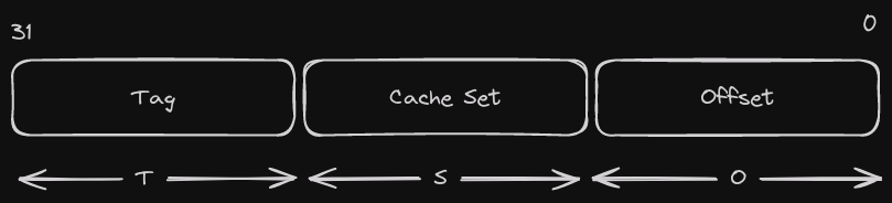
Offset O = log~2 (cache line size)
Cache Set S = log~2 (number of sets)
Let's take this simplified system to understand this better:
- L1d cache of 512 bytes
- Each cache line is 64 bytes, that means 8 cache lines (512/64)
- A 2-way set associativity
So for the above system:
Number of sets = (cache lines) 8 / (associativity) 2 = 4
O = log~2 (64) = 6, S = log~2 (4) = 2
O = 6, S = 2, T = 32 (or 64) - S - O
If you are a visual learner, this video does a pretty good job of explaining how addresses in memory are mapped to the cache.
This is important to know, when you run micro benchmarks as the size of the block can vastly change the performance, based on how it fits into the cache. For more details (Read #91 of 100 Go mistakes).
So how does effectively using the cache line effect the performance of programs
I'm going to use a very simple example of traverse through an array in two different ways:
Row Major
func RowMajorTraverse(arr [rows][cols]int) {
	for r := 0; r < rows; r++ {
		for c := 0; c < cols; c++ {
			arr[r][c] += 1
		}
	}
}
Column Major
func ColumnMajorTraverse(arr [rows][cols]int) {
	for c := 0; c < cols; c++ {
		for r := 0; r < rows; r++ {
			arr[r][c] += 1
		}
	}
}
The change is code minimal but the difference in performance in quite significant. These are the benchmarks on my machine:
test -bench="BenchmarkRowMajor|BenchmarkColumnMajor" -count=5
goos: linux
goarch: amd64
pkg: bench
cpu: Intel(R) Core(TM) i7-7700HQ CPU @ 2.80GHz

BenchmarkRowMajor-8      	     778	   1496554 ns/op
BenchmarkRowMajor-8      	     748	   1668281 ns/op
BenchmarkRowMajor-8      	     720	   1530100 ns/op
BenchmarkRowMajor-8      	     765	   1521765 ns/op
BenchmarkRowMajor-8      	     756	   1508556 ns/op

BenchmarkColumnMajor-8   	     444	   2609167 ns/op
BenchmarkColumnMajor-8   	     444	   2638403 ns/op
BenchmarkColumnMajor-8   	     454	   2617205 ns/op
BenchmarkColumnMajor-8   	     450	   2616833 ns/op
BenchmarkColumnMajor-8   	     448	   2620201 ns/op
This is a very simplistic example, but the idea is how two identical looking code can have such significant differences in performance.
More code examples
If you would like detailed examples and explanation check our, Go and CPU Caches by Teiva Harsanyi is an excellent source. For examples in C, you can follow the ones in the paper above by Ulrich Drepper.
Finally
To conclude, I haven't completely read the paper yet, it took me some time to understand the bits I have read so far. I plan on reading the complete paper over the next few weeks. The paper even though quite old (from 2007) still helped me understand code optimizations from books that were written a couple of years ago (2022). More importantly, it provides much needed mechanical sympathy required to write more efficient and effective software.
I found this paper as I was watching this talk from 2014, which is a great starting point and might inspire you to read the paper yourself.